
By Leslie Nemo
It took four days in 1913 for the future of the Miami Valley in Ohio to change forever. Starting on March 23, roughly 10 in. of rain fell on ground that was already saturated from melting snow and ice. The stretch of the Great Miami River meandering through the southwestern part of the state began to overflow, flooding a constellation of surrounding cities. More than 360 people died and property damage exceeded $100 million ($3 billion in today’s economy), according to the Miami Conservancy District website.
“A large share of the blame for the resulting damage must be laid to man ... because of the entire absence of any comprehensive engineering works built for the prevention of such damage by floods,” wrote A.H. Horton and H.J. Jackson in the 1918 U.S. Geological Survey report, “The Ohio Valley Flood of March-April, 1913,” which assessed the outcome of the flooding.
Ohio towns like Hamilton and Piqua organized individual construction programs within days of the disaster. Dayton did too, creating a flood prevention committee on May 2, 1913. Led by local industrialists John Patterson and Edward Deeds, the organization fundraised $2 million, part of which was to be spent on an engineer.
The committee landed on Arthur E. Morgan for the job. Morgan, a college dropout, learned the ins and outs of drainage solutions from his civil engineer father, John. By 1913, Morgan had been running his own engineering company out of Memphis, Tennessee, for several years and was known for his specialization in drainage engineering, wrote Aaron D. Purcell in “Reclaiming Lost Ground: Arthur Morgan and the Miami Conservancy District Labor Camps” (The Historian, Vol. 64, No. 2, Winter 2002).
In the summer of that year, Morgan and his engineers and surveyors set out across the Miami Valley to assess the scope of the work. The report Morgan delivered in early October to Dayton’s committee concluded that widening the river channel would not be enough to prevent future catastrophes. Instead, Morgan recommended channel improvement measures along with the construction of five reservoirs or dry dams (with hydraulic-fill cores) stationed along the Great Miami River channel. Only when the valley flooded would the dams hold water, according to Purcell.
Morgan’s suggestion was communal — if one town needed the network of dams to avoid local disaster, then all Miami Valley municipalities needed to cooperate for the project. Ohio state law did not allow for projects to stretch across local governments, so a Dayton representative brought the Conservancy Act of Ohio to the state legislature. Passed in February 1914, the law permitted flood control agencies to build and run infrastructure in multiple communities. Lawsuits challenging the constitutionality of the bill proceeded until late in 1917 when the Supreme Court of Ohio deemed the act was lawful. When the legal opposition wrapped, the newly minted Miami Conservancy District was free to start construction.
Morgan and his crew of nearly 50 hand-picked civil engineers decided dam construction would proceed simultaneously in each location. Every site had a “gravel washing and screening plant” to supply aggregate for concrete as well as a cement storage facility, hydroelectric plant, and power distribution station, according to Chas H. Paul in his 1925 book Construction Plant, Methods and Costs: Technical Reports Part X.
The district originally planned to hire contractors but opted instead to bid out the work in 1917 — in the middle of World War I, when labor was challenging to find. When the applicants proved scarce and expensive, the district decided to do the work itself, hiring its workers directly and buying its own equipment, including 21 dragline excavators. The technology was so crucial to the work — and so novel — that Paul dedicated an entire chapter of his book to the machines. The excavators were particularly useful for carving borrow pits into gravel beds that sat below water level.
With equipment at the ready, construction began in 1918. The district engineers decided hydraulic fill — a method by which sand is excavated from one location, deposited in another by using water to move it, and then the water is drained off — would be the best construction method for each dam, despite the broader skepticism others had of the technique.
“The hydraulic method of dam construction has great advantages, but too many dams built by it have failed,” wrote Allen Hazen, M.ASCE, in a 1919 issue of the Transactions of the American Society of Civil Engineers (Vol. 83, No. 1). To avoid this fate, Morgan and his team drew samples from possible borrow pits throughout the valley and had the U.S. Bureau of Soils compare them with extractions from other hydraulic fill dams.
The engineers also sought to gauge how well the dam cores would solidify. Their solution was the Goldbeck earth pressure cell, which they had read about in reports from the U.S. Department of Agriculture. The Miami team contacted the federal lab, and A.T. Goldbeck, the inventor of the device, went to Ohio to help install his designs.

In Construction Plant, Methods and Cost, Paul described the cell in this way: “Briefly, the Goldbeck cell is a closed, flat, circular box, 5 1/2 inches in diameter, similar in shape to a shoe-blacking box, the top or bottom of which acts as a movable diaphragm.” As each dam grew in height, workers buried the flat Goldbeck cells at different elevations. Some went in horizontally, others vertically.
Compressed air was forced into the cells via small pipes. As the embankments got taller, the weight of the dams pressed the lids of the boxes into place, closing an electrical circuit. Engineers could gauge the amount of pressure building inside the structure by pumping air into the boxes. When the internal air pressure equaled the external dam pressure, the lid on the box would lift enough to break the circuit and turn off the indicator light, according to Paul in “Core Studies in the Hydraulic-Fill Dams of the Miami Conservancy District” (Transactions of the American Society of Civil Engineers, 1922, Paper No. 1502).
The readings from the horizontal and vertical boxes showed that vertical pressures eventually surpassed lateral pressures. “The Conservancy dams are the first in which such cells have ever been applied to such a purpose,” wrote an unknown author in the April 1920 issue of the Miami Conservancy Bulletin (Vol. 2, No. 9). “The first, in fact, in which any consistent attempt has been made to know, as the work goes on, just what happens to the core materials.”
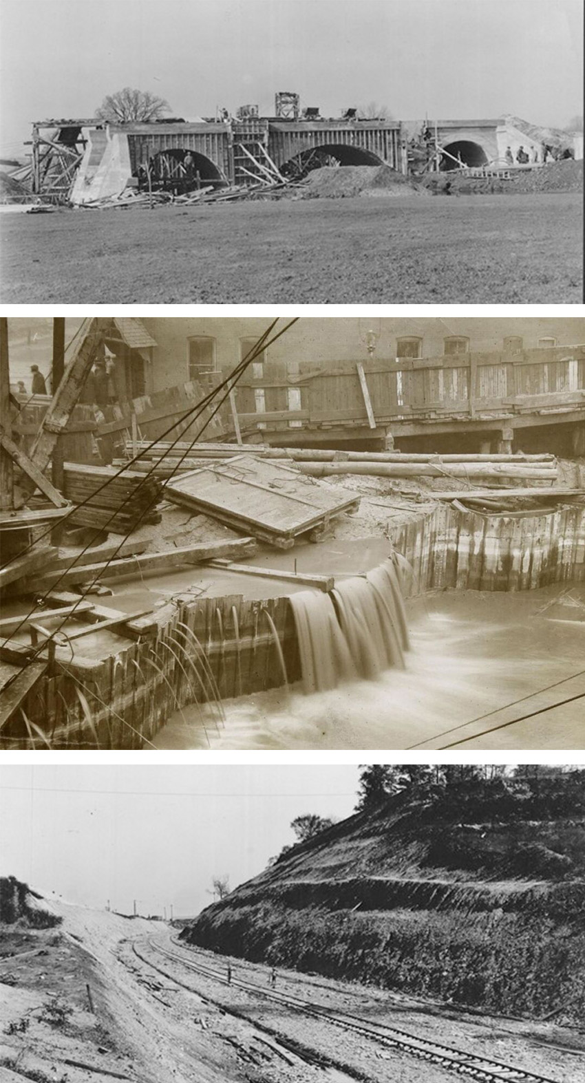
The favorable pressure readings boosted district confidence as two dam designs were implemented across the valley. The first approach, as seen in the Germantown and Englewood dams, relied on pairs of concrete horseshoe conduits going through the earthen embankments. To make sure communities were not flooded during the work, the district team built the conduits first — and to depths that the team later filled in and reduced — so that the channels could handle any flooding experienced before the rest of the construction finished.
The Germantown Dam, the sole structure south of Dayton, was made of 835,000 cu yd of material, 800,000 cu yd of which was placed using the hydraulic fill method. The valley site was too narrow for temporary spillways, so over the course of a summer, the time of year the team deemed least likely to experience flooding, teams had to get the embankment to a height tall enough to stave off flooding with help from the conduits.
The Englewood Dam, which was 10 mi north of Dayton, was the biggest and tallest (124 ft tall at its maximum) of the five dams. Made from 3.6 million cu yd of material, all but 200,000 cu yd came from hydraulic fill. Borrow pits extended for about 1 mi alongside the dam and reached almost a third of a mile across in some places, wrote Paul in Construction Plant, Methods and Cost. However, unlike Germantown, this dam was too large to build up sufficient embankment height in one season. Instead, workers created the conduits while starting a hydraulic fill structure on the opposite side of the river.
The next summer (1919), the team closed off the river and raised the hydraulic fill embankments high enough that they could divert any flooding into a temporary spillway. Only in 1920 was the fill high enough that the spillway could be removed.
Elsewhere across the valley, workers completed the second dam design. Whereas the Germantown and Englewood dams had spillways far away from their outlet conduits, the Lockington, Huffman, and Taylorsville dams merged the two features into a single location. Concrete floors at the level of the riverbed connected to two parallel retaining walls. Sandwiched between the vertical structures was an ogee overflow spillway with conduits at the base.
The Lockington Dam put this design to use 5 mi north of Piqua. The longest of all the dams at 6,400 ft, the two-conduit design was also on the shorter side. “A considerable portion of the dam at either end is nothing more than an earth levee 15 feet or less in height,” Paul wrote in Construction Plant, Methods and Cost. Of the 1 million cu yd of fill used to build the dam, 795,000 cu yd was deposited by hydraulic fill, sluiced from a higher elevation upstream.

The Huffman Dam was constructed 8 mi east of Dayton. At 73 ft tall and with a volume of 1.396 million cu yd, the Huffman structure had three outlets. While not the biggest or smallest dam on the project, it was possibly the most frustrating. The construction schedule had to navigate relocating three railway lines that went through the area. And though the dams would never hold water permanently, the town of Osborne sat in the Huffman flood zone. So to protect their homes and businesses, from 1922 to 1925 residents moved every building 2 mi south.
The Taylorsville Dam site was one of the last to be completed. Nestled into a valley 10 mi north of Dayton at 78 ft tall, the outlet installed here was the project’s largest concrete structure. Its four conduits are flanked by two retaining walls reaching about 90 ft tall. Workers built up much of the embankment first, drawing on some of the material carved out for the conduits. The dam site abutted Cincinnatian rock, so some excavated material had too much shale and hard clay to work as fill. Nevertheless, it could not go to waste, so the team placed it on the toes of the embankments upstream and downstream.
Meanwhile, construction teams fixed minor mistakes made in the pressure cell installations at other locations. Some air pipes developed leaks, while wooden support towers installed to hold the cells suffered structurally because the foundations sat in solidified material while the tops moved as upper fill started to settle. So at Taylorsville, the cells were attached instead to the concrete retaining wall, while larger, airtight pipes fed them air. “The results to date have every indication of being reliable,” wrote Paul in his Transactions article.
A couple of happy accidents along the way also reassured Morgan and the district team of their dam designs. With about 12 ft of construction left to go at the Lockington Dam embankment, the core pool overflowed. The runoff carved a depression into the slope of the dam exposing the core. Only about 10% of the solidified core moved with the runoff, and in the 3-4 weeks needed to repair the gap, the engineering team did not notice any sloughing of the core.
Workers also used the opportunity to carve away more of the dam face to take a core sampling in what Paul called a “biscuit-cutter fashion.” Each segment showed a low moisture content hovering around 23%. A similar accident (and results) played out at Englewood. “In the face of the evidence offered by these core exposures, there is no doubt that consolidation of these cores has progressed at a highly satisfactory rate,” Paul concluded in his Transactions article.
The district announced the project’s completion on April 17, 1923, though the construction on all aspects of the $30 million (more than $500 million today) flood protection system wrapped before the end of 1922, according to the district’s website. By then, the dams had consumed 8 million cu yd of earth and more than 160,000 cu yd of concrete. Channel improvements, including straightening, deepening, and cleaning, required crews to excavate 5.3 million cu yd of material. Furthermore, about 50 mi of railway was shifted to make room for the dams, Paul wrote in his book.
The first major test of the infrastructure came during a 12-day period in January 1937 when the amount of rainfall equaled the epic four-day rainfall in 1913. All the dams and levees worked as expected. As of the end of 2021, the dams had collectively kept floodwater at bay 2,085 times, according to the Miami Conservancy District.
If the original project engineers felt confident when their dams passed core sampling and cutting-edge pressure detection tests, then they would be pleased to hear the structures have so far passed the test of time.
The Miami Conservancy District was named a National Historic Civil Engineering Landmark in 1972.
Leslie Nemo is a journalist based in Brooklyn, New York, who writes about science, culture, and the environment.
This article first appeared in the November/December2023 print issue of Civil Engineering as “The Miami Conservancy District Proves a Point.”